Pandas+Seaborn+Plotly:联手探索苹果 AppStore
公众号:尤而小屋<br>作者:Peter<br>编辑:Peter
大家好,我是 Peter~
今天给大家分享一篇 kaggle 实战的新文章:基于 Seaborn+Plotly 的 AppleStore 可视化探索,这是一篇完全基于统计+可视化的数据分析案例。
原 notebook 只用了 seaborn 库,很多图形小编用 plotly 进行了实现,原文章地址:https://www.kaggle.com/adityapatil673/visual-analysis-of-apps-on-applestore/notebook

导入库
数据基本信息
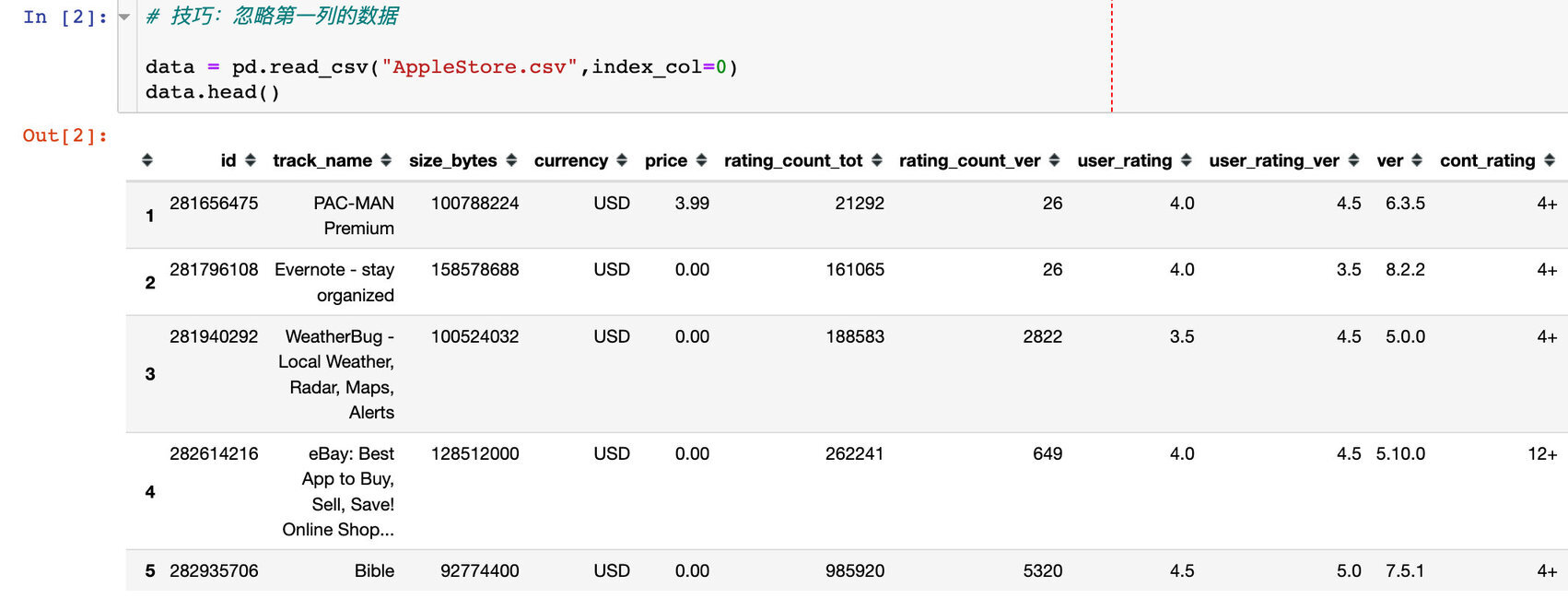
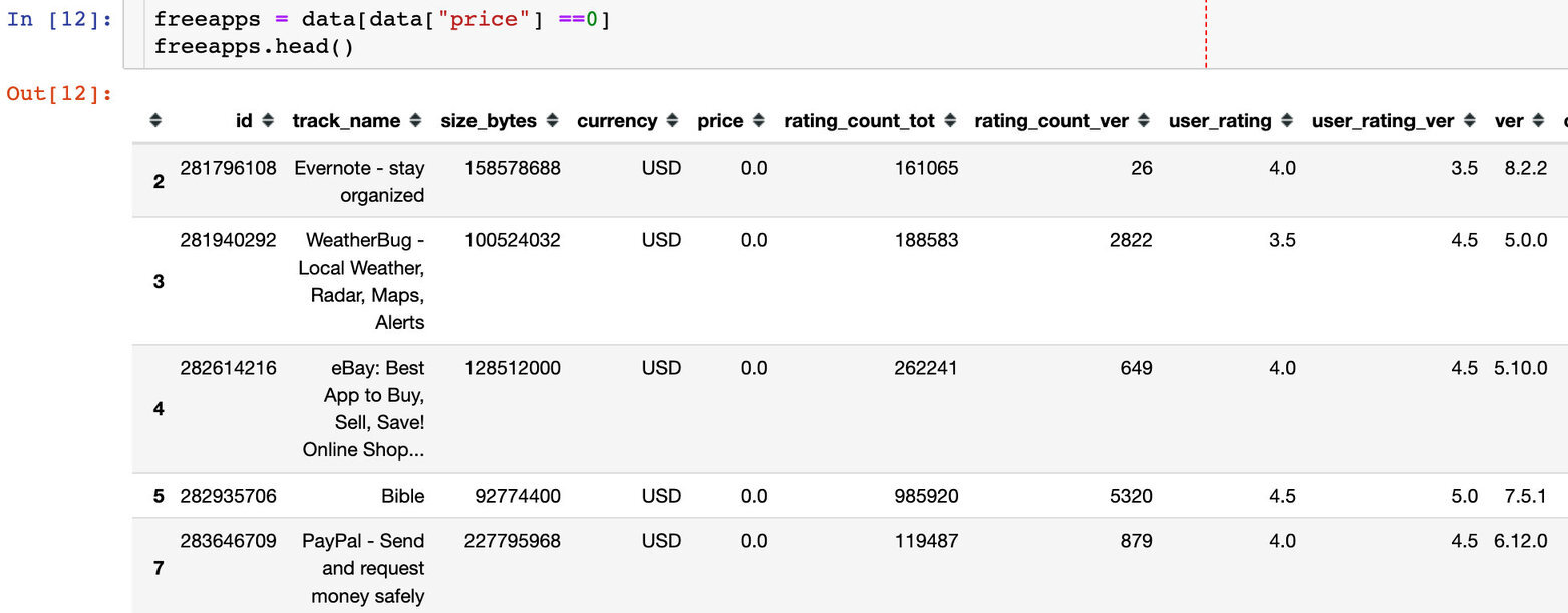
读取并且查看基本信息:
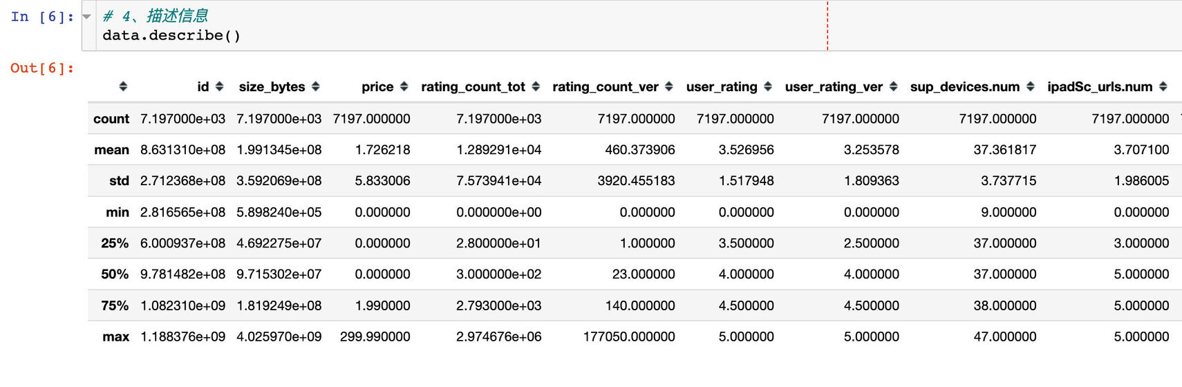
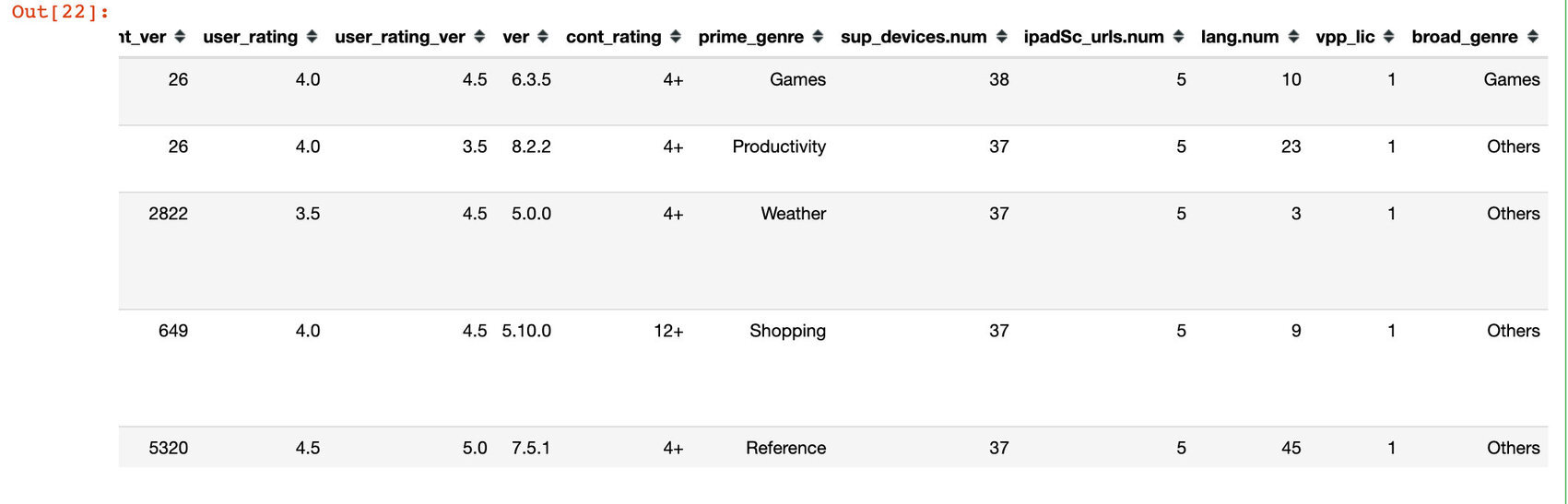
一般情况下,也会查看数据的描述统计信息(针对数值型的字段):
APP 信息统计
免费的 APP 数量
价格超过 50 的 APP 数量
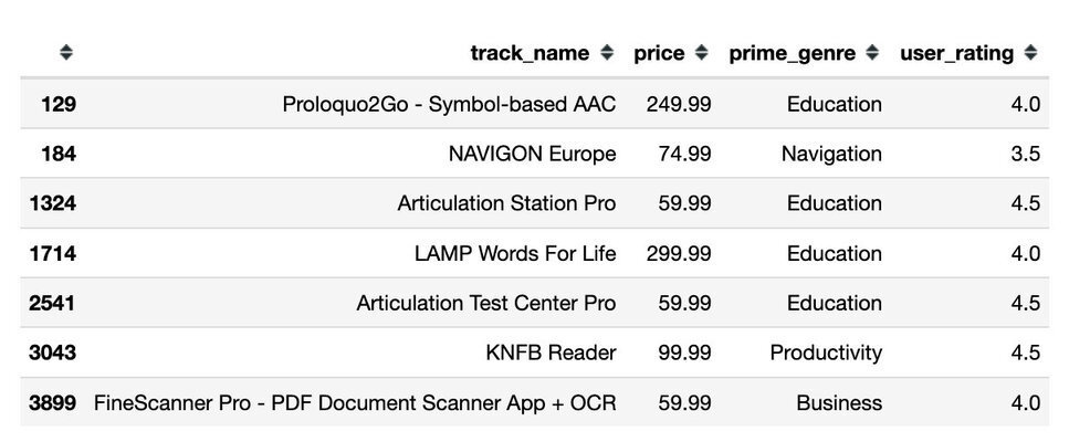
价格大于 50 即表示为:超贵(原文:super expensive apps)
价格超过 50 的比例
离群数据
价格超过 50 的 APP 信息
免费 APP
选择免费 APP 的数据信息
正常区间的 APP
取数
价格分布
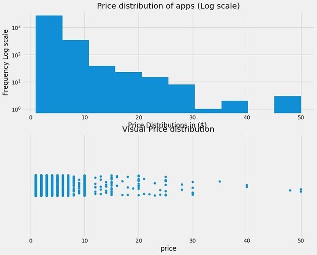
结论 1
随着价格的上涨,付费应用的数量呈现指数级的下降
很少应用的价格超过 30 刀;因此,尽量保持价格在 30 以下
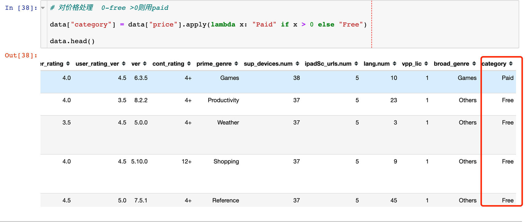
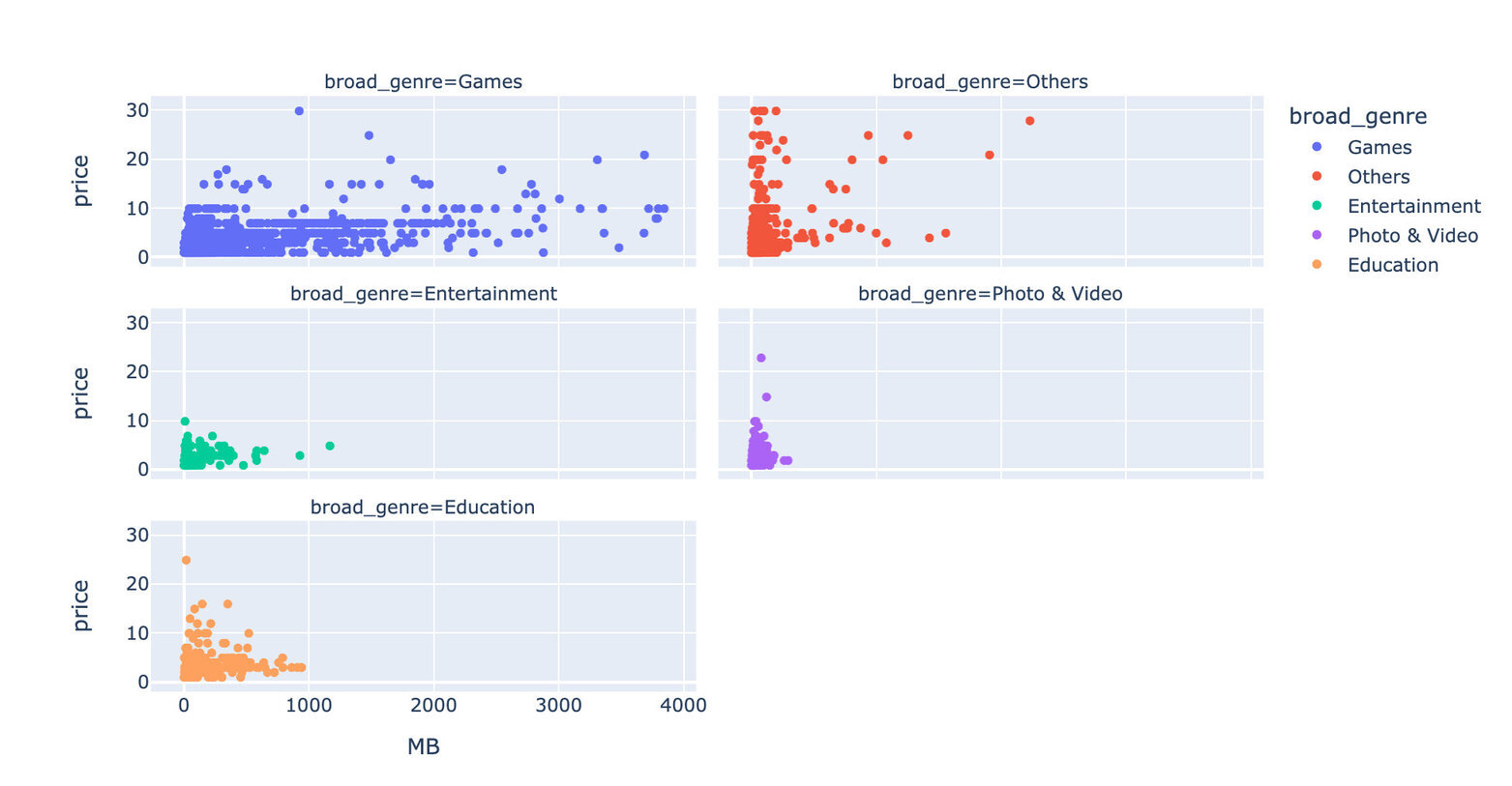
category 对价格分布的影响
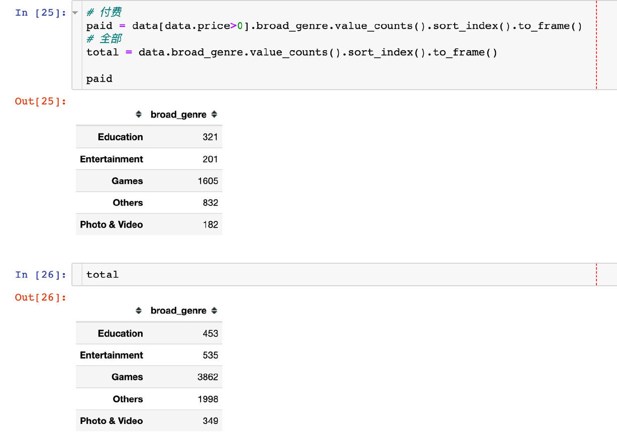
种类及数目
显示前 5 个种类
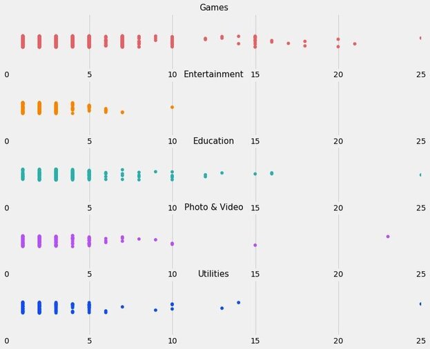
结论 2
Games 游戏类的 apps 价格相对高且分布更广,直到 25 美元
Entertainment 娱乐类的 apps 价格相对较低
Paid apps Vs Free apps
付费 APP 和免费 APP 之间的比较
app 种类
选择前 4 个
选择前 4 个,其他的 APP 全部标记为 Other
统计免费和付费 APP 下的种类数

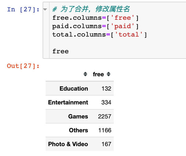
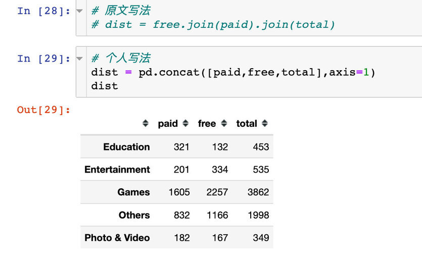
将两个数据合并起来:
统计量对比
高亮显示最大值(个人增加)
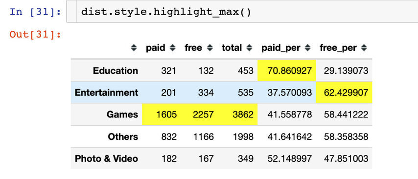
结论 3
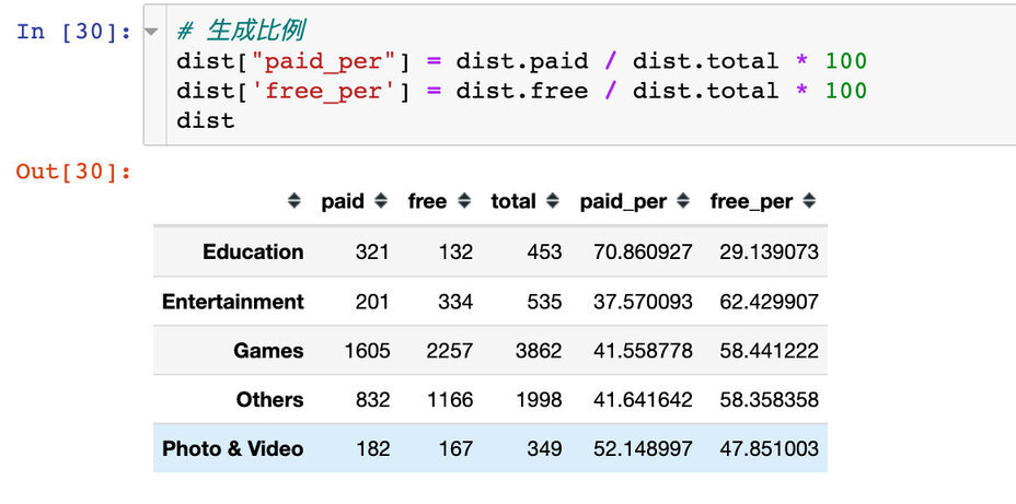
从上面的高亮结果中,我们发现:
Games 相关的 APP 是最多的,不管是 paid 还是 free
从付费占比来看,Education 教育类型占比最大
从免费占比来看,Entertainment 娱乐类型的占比最大
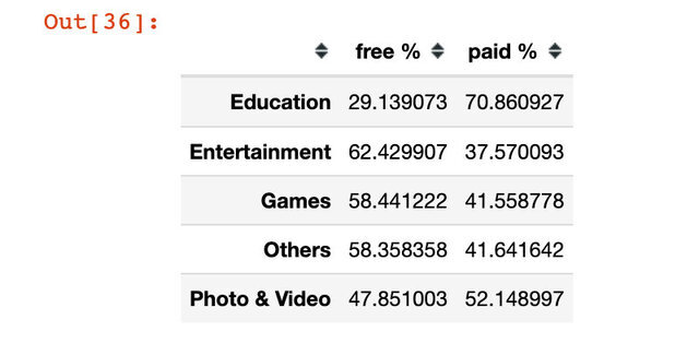
付费和免费的占比
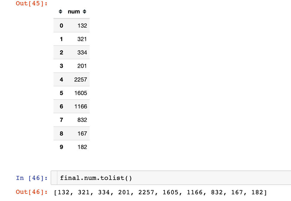
生成数据
分组对比付费和免费的占比
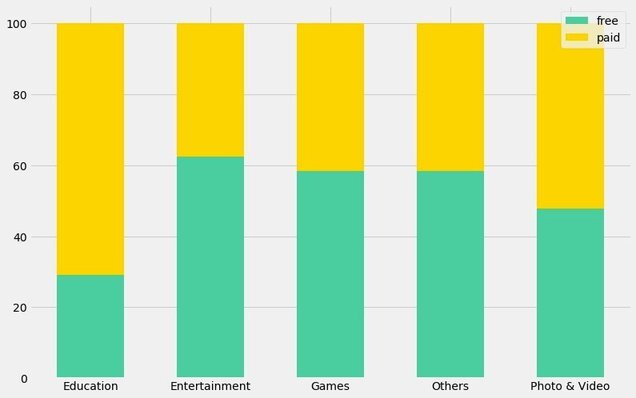
柱状图
饼图
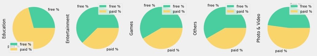
结论 4
在教育类的 APP 中,付费 paid 的占比是很高的
相反的,在娱乐类的 APP 中,免费 free 的占比是很高的
付费 APP 真的足够好吗?
价格分类
小提琴图
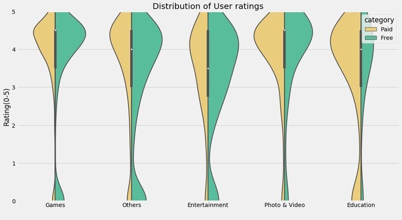
结论 5(个人增加)
在 Education 类的 APP 中,paid 的占比是明显高于 free;其次是 Photo & Video
Entertainment 娱乐的 APP,free 占比高于 paid;且整体的占比分布更为宽
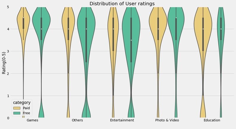
注意下面的代码中改变了 split 参数:
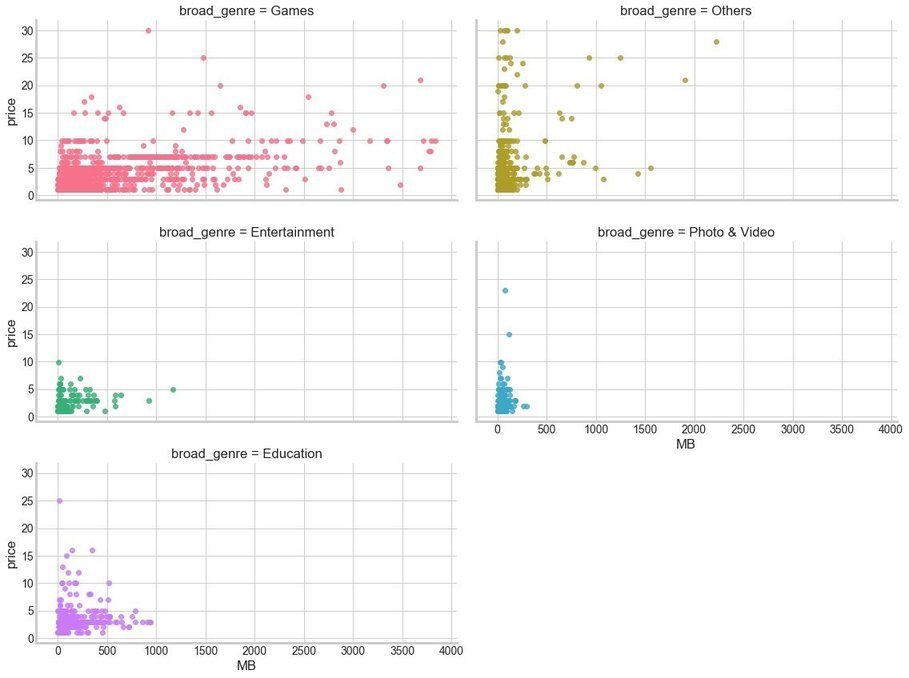
size 和 price 关系
探索:是不是价格越高,size 越大了?
使用 Plotly 实现(个人增加)
增加使用 plotly 实现方法
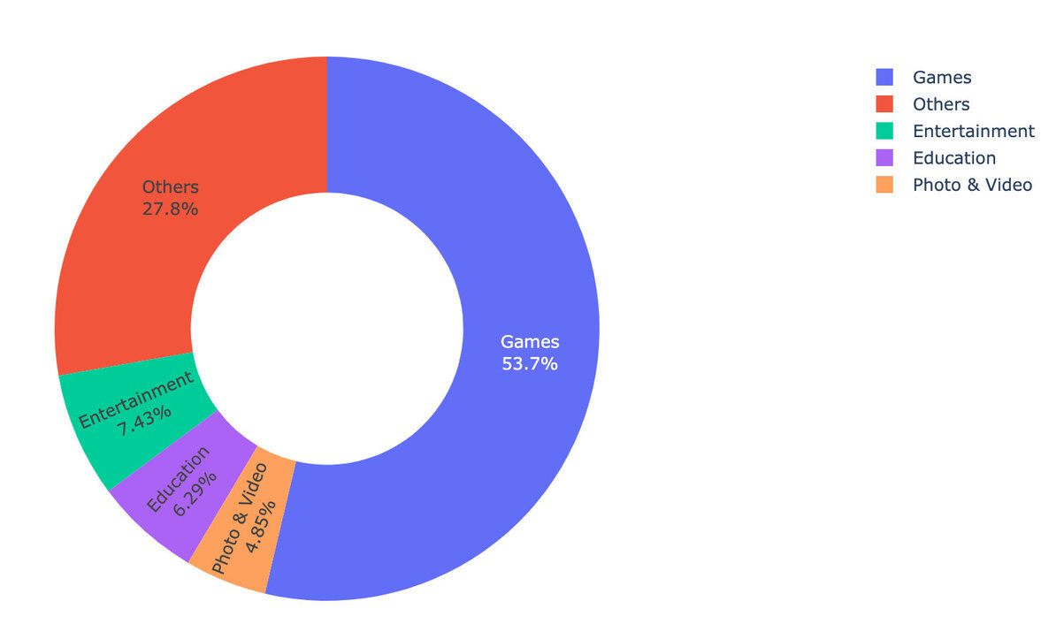
APP 分类:是否可根据 paid 和 free 来划分
5 种类型占比
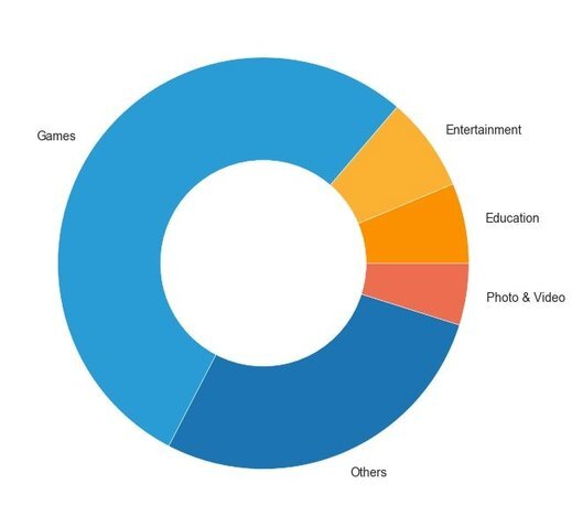
使用 plotly 如何实现:
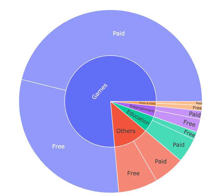
5 种类型+是否付费
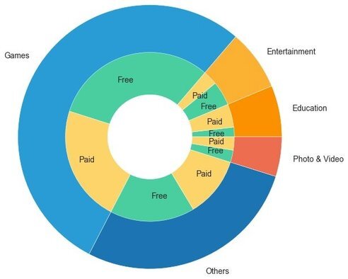
基于 plotly 的实现:
版权声明: 本文为 InfoQ 作者【Peter】的原创文章。
原文链接:【http://xie.infoq.cn/article/20c95f1355b6ae13ec69a9755】。文章转载请联系作者。

志之所趋,无远弗届,穷山距海,不能限也。 2019.01.15 加入
还未添加个人简介


评论